Seeking updates for the next MADByTE patch

Hello Everyone,

I am seeking updates that you wish were in MADByTE to help bolster our next release:

  • Are there issues with getting your data into MADByTE?

  • Is there unexpected behavior that you find troublesome?

  • Is it a pain to use?

Any feedback you have, please don’t hesitate to create an issue on the Github page (https://github.com/liningtonlab/madbyte/issues) and I’ll we’ll do our best to address them!

Problems with MADByTE on a Mac?

While preparing our latest manuscript, I found a problem with the new M1 Macbooks running MADByTE:

They didn’t run it.

So, after some panic about what could have gone wrong, I noticed that the GUI infrastructure that MADByTE uses has a bit of a problem running on apple silicon. So, I updated the pyqt5 package and verified it ran.

Then, just a few days ago, it stopped running… again..

So, remembering this issue, I found that once again the M1 Macbooks had updated beyond what the fixed version of pyqt5 we recommend was. Once again, I updated the pyqt5 version and we’re back in business.

So, if you’re struggling to get MADByTE to launch, try updating pyqt5 first. If the problem persists, feel free to reach out to me directly and I’ll work with you to figure out what may be going wrong. We’ll try to keep the repo up to date, but if it isn’t - just let me know!

Tackle your data storage in Topspin

Bruker has been hosting some fantastic webinars on getting to know their software and instruments during the COVID-19 shutdown (Found here). There are some fantastic little tips that come out of these webinars that to the average student (with only a few years of experience, and mostly with automated collection) may find confusing or duanting…This is not one of those tips.

Working with 2D Metabolomics data can be quite difficult, since the amount of data collected, processed, and stored can increase quite quickly. In the words of Clemens Anklin from Bruker during the tips and tricks webinar:

NMR Data is like a noble gas, it will expand to fill all available space

So how can we reduce the impact of our data on our storage? The problem is real, but the solution is imaginary. When you process your NMR data, especially NUS data, the file size jumps quite quickly because you are using the real and imaginary part of the data to process. However, once your processing is done, the imaginary serves little to no purpose for most users - so we can discard it.

To do this, open a file in Topspin from the directory you wish to condense. In this case, I have a folder which is for a completed project- perfect! Let’s see how we can cut down on storage:

Starting directory size: 7.33GB

Opening a data file from my “Biomap Active” project, I then type “deli”. Although it sounds like I’m trying to have topspin reconstruct a sandwhich, it stands for delete imaginary. This then launches the following menu:

Capture.PNG

Since I don’t need any of this imaginary data at the moment, I select all the files and hit ‘ok’. There is no confirmation and it doesn’t take very long, but…

New directory size: 2.03GB.

If you ever need the imaginary part of the data back, you can simply re-calculate it by doing a hilbert transformation - type ‘xht1’ and/or ‘xht2’ to reconstruct it if you need it.

Using Au Scripts To Automate Topspin

Automation scripts in Topspin are coded as C language based scripts. This differs from python style scripts significantly, and has its advantages and drawbacks like any programming language. Without making too many comments on preferences, I will say that I do not know much about C languages, except some basic differences (such as having to define what kind of value a variable will stand for, explicitly). As is the case with python and macro scripts, you will need to navigate to the edit screen to find these codes - but this time with edau.

  • Commands are typed in bold - edpy/edmac/edau

  • Variables are in italics - i1

The good news is that much like the macros and python, many commands that you would use in topspin are already coded in as commands you can call directly. This means that if you wanted to clone our macro into an automation script, you can do that! In fact, a few of the commands you may already use already ARE automation scripts! As an example, lets pull up one of the many provided scripts, multizg.

If you are using a spectrometer without IconNMR or the spooler service activated, you may be familiar with multizg.. but what does it actually do? Navigate to the Burker script directory with edau and find the multizg script.

From the description in the au file, you can see that multizg program written by Rainer Kerssebaum contains a few blocks of code to allow for multiple experiment acquisition. If you have set up experiments beforehand (10 -1H , 11-HSQC, 12-TOSY) then when you activate multizg and enter in the correct number of experiments, it will read each file and run the acquisition. If you haven’t set up the experiments beforehand though, it will simply copy the open acquisition and run that many of that particular experiment – this has caught me a couple of times...

If you look at the way it iterates through the experiments, it prompts the user for the value of ‘i1’ which can be thought of as the number of experiments to be run. If i1 > 0, as it should be, then it calculates the number of experiments that are queued up and the experiment time for each. Once that has been completed, it iteratively runs through the experiments until all of them have been completed. Pretty cool right? Now, this is a very advanced script, and it looks pretty dense to a new user – DON’T PANIC. Lets try to write a very simple Au script to do some 1D processing. As you get more comfortable, try writing some more cleaver Au scripts to perform your tasks for you!

Sticking to the command line arguments, simply write a new Au script called 1D_ZG. Assuming we’ve set up the experiment correctly and it is open, let’s write a script to set the receiver gain and then acquire the data.

1D_ZG.PNG


Unlike Macros and Python scripts, Au scripts must be compiled before they can be executed. Select “Compile” and after a few seconds, you will get a prompt that tells you it’s ready to go! If you have errors or language in there that confuses the system, it will give you a kickback message that tells you something is incorrect. Au scripts offer the users who are familiar with C based languages a chance to put their skills to work for them, and it’s a fantastic option. Try looking through some other provided scripts, such as the pulsecal script, to get a better idea of how to interact with Topspin.

If you were lucky enough to catch the advanced Topshim webinar by Bruker, you might have seen how you can further expand our script to include specific shimming steps as well, further automating your acquisition step. As is the case with all three types of automation, once you have these scripts established in your directory, you can simply call them up using the command line - or even code in your own buttons!

Using Python To Automate Topspin

Topspin contains a very powerful tool for automation – Python. If you aren’t familiar with python, what you should know is that it is extremely easy to pick up, it generalizes very well, and is coding is done ‘in plain english’. By ‘plain english’ I mean that it is very simple to get started compared to other coding languages. In the interests of time, I won’t be going into python, there have been countless tutorials on that posted to youtube, and I simply can’t compete or offer insight into anything better than they can.

Assuming you’ve used Python, you’re in great shape to begin processing your data through topspin. Luckily, topspin installs a native python so that you can begin working with it without having to pull yourself into ‘which python’ territory.

Let’s get started!

  • Commands are typed in bold - edpy/edmac

  • Parameters are in italics - TD/SI/LPbin

First, we need to open the python module in Topspin. We can do this by simply typing ‘edpy’ into the command line. This brings up a menu allowing you to see some sample python scripts that Bruker has included. For now, lets pull one up and take a look at how we may be able to use this. Perhaps one of the best scripts to get you started would be the ‘py-test-suite’ script.


In this script, we can see that we define some dialog boxes – but importantly, these dialog boxes are defined using topspin specific commands that do not exist in standard python and there are many other commands that are hard coded into topspin python.  Bruker’s team has done a lot of work for you already!

As is the case with the last lesson, we are going to design a python script to automate something we already do – in this case we’ll be performing some linear prediction and zero filling, reprocessing the data, and peak picking. For this demonstration, we are going to use linear prediction in both dimensions, although this is usually not done since we can normally acquire enough points in F2 to not need it.

Some basic steps still apply, we are going to create a new python script for this, but in order to do so, you must switch the python module directory to the' “…../py/user” directory in the edpy menu. Once there, select new and give your new masterpiece a title.

This opens up a built in notepad that we can code in and execute the script from directly. This is useful for testing whether a command works or not, so I constantly click that execute button. You’ll notice the “Warn on Execute” button there…I’d disable it when troubleshooting, since it sends a pop-up your way every time you test the code out.

Start_Of_SI_TD.PNG

In this first chunk of code, we are simply retrieving the values for the parameter TD from the OPEN dataset. Next, we use a built in dialog box to send a message to the user about what those parameters actually are, and then do the same for SI. You may notice that I tell the script to convert the value of TD1 and TD2 to strings using the str() command. This is actually not required, since the GETPAR( ) function returns values as strings, but I choose to force the hand.

Using these values, we then simply multiply the TD by 2 to find a viable SI value which will allow us to do both linear prediction and zero filling. In order to do this, however, we need to remember that the value of TD1 and TD2 are given as strings - so we tell python to convert that string into an integer. Here, you notice that when we are setting the value, I’ve changed the convention from GETPAR(parameter,axis=XYZ) to PUTPAR(‘axis# variable’, value). You can retrieve the values from GETPAR using this convention as well if you desire.

Placing_Vals_py.PNG

Once our new SI values are set, we want to tell the system that we plan on using linear prediction, and what kind. We do this by setting the ME_mod parameter to “LPfr'“ (which stands for linear prediction in the forward direction using real points) using the same conventions we used earlier. Then, we multiply TD1 and TD2 by 1.5 to give us the extrapolated points we wish and we store those values as LPBin values for each axis. The remaining points that are not accounted for by LPbin or TD are zero filled automatically.

LP_Bin_pyu.PNG

Now that we have all of the relevant values set, we are ready to process the spectrum using our new settings. This can be done using a built in command as well, simply XFB( ). However, let us assume that this command WASN’T hard coded into topspin. In this case, there is a lovely function called XCMD( ) where you simply type in the command you would use in the command line. In this case, we would use XCMD(‘xfb’) to perform this action.

xfb_py.PNG

After this, we have our new spectrum returned with linear prediction and zero filling performed. We could end there, but there is one more feature that you might like to know about. Using the built in functions, some of them can be passed variables or commands that alter the way the function is performed. Take, for instance, peak picking. If we were using this script to do automatic peak picking on the spectrum, the last thing we want is to have the peak picking dialog box pop up for each of our 100 samples - so we' disable the pop up box by instead opting for the silent mode of peak picking.

pp_py.PNG

And voila!

As you can see, the python option allows you to manipulate data in a very similar manner to the Macro’s, but also allows for a bit more control. For instance, there are even options to browse through all your data to selectively process things. It also allows you to pull data into the script and compare directly - handy for dereplication if you have a library… I’ll post a tutorial in a few weeks showing exactly what I mean by that, as well as a lovely little function I’ve created that allows for semi-supervised peak picking of metabolomics data.

Although there does exist explicit documentation for using python in Topspin, I’ve found that I wish it had a list of all of the built in functions that was readily accessible. However, they do offer about 15-20 pages on selective use cases, so it’s a good start.

Getting Started With Macros In Topspin

Macros are the most basic processing schemes available to a user in Topspin, and provide a great level of automation with very basic skills. Simply put, a well designed macro could automate a large portion of your workflow, allowing you to process data in your sleep.

It is overly simplistic, but for the sake of this quick start guide, think of each line of a macro as the command line at the bottom of Topspin. When you open your data, you use commands in this line for basic transformations of the data, editing processing variables, and even adjusting the viewing window. These commands can have variables passed to them in the command line as well, which is how we should think about them in a processing macro.

Lets take a simple example of 1D data – using only the command line to process it. Then, we’ll write a macro which will do the same transformations on the data, and finally, we’ll link it to the Topspin “serialcommand to automate processing for multiple datasets.

(Find the dataset here)

Command Line Processing

When we open this dataset, we need to transform it first. For this, we use the line command “ft”. Once we have a spectrum, we can see that we need to apply phase correction. If we use automated phase correction, the command for 1D data is “apk”. Next, we perform baseline correction without integration by “absn”. Following these three commands, we have processed our data to the point an investigator might begin looking at the spectrum for peaks of interest. There are, of course, other commands and combinations – depending on what your processing scheme might be. As an example, if you wish to include integration into this scheme, you have three choices. You can either change the commands fed into the system – replacing “absn” with “abs” which uses automatic integration, you can implement integration in another step, or you can choose to integrate the spectra yourself. Hopefully, you can see the flexibility of having all three options available, depending on your application.

Since you have to perform these basic functions on every spectra, why not construct a macro that would do it for you with an easier command? These few seconds you save may not seem like much, but with even a 3 second savings per spectra, a sample size of 100 samples processed could save you more time than you spend writing the macro: so lets do that.

Writing and Editing Macros

First, you have to open up the Macro menu in Tospin by typing the command “edmac”. This launches the Macro menu, likely populated with a lot of Bruker provided scripts that automate a large chunk of processing. First, lets look one of the provided examples, the example_efp macro – open this up by highlighting the script and selecting edit.

Burker_Macro_Example.PNG


By selecting edit, you launch the macro edit utility, which is similar to a idle processor/notepad. By looking at this example, we can see that – much like python – we can write notes alongside commands by using the # sign before writing in a line. As the program moves down the line, these lines are ignored completely, allowing you to leave a detailed explanation of each step – or slip in some user information or metadata about the sample sets you are writing the macro for. Keeping highly detailed coding notes is a VERY SMART MOVE. The line structure of the Macro allows you to command the program to do one task, and when it is complete, it moves on to the next task. Dissecting the example script above, we can see that it uses a similar approach to basic processing:

·       Perform exponential window multiplication with “em”

·       Perform Fourier transformation with “ft”

·       Perform phase correction with “pk”

For the sake of this quick start, we’re going to start fresh and write our own script. In order for us to edit or create a new macro, we need to change the source directory where topspin is looking for our macros. By default, this normally opens to the bruker directory (C:…..expt\stan\nmr\lists\mac) – to navigate to your directory, simply select the drop down menu and select the (…mac\user) version of the directory. If you’ve never experimented with Macros, this will be empty. Select File > New. Here, you’ll be prompted for a name, which can change later. For now, let’s name this something easy – ‘JE_tut1’.

Tut1_Fresh.jpg

Lets try writing a quick macro to do the commands we outlined on our 1D data – ft, apk, absn. Once we’re done, you can simply click execute to test the command – if it processes without flagging an error, it worked!

tut1_simple.jpg

If you’re satisfied with the macro, you can save it and recall it any time with a variety of different methods. My favorite, is the ability to call on a macro/script/python script by simply using it’s name in the command line. Try it by saving the script, exiting out of the macro window, and typing “JE_tut1” in the command line. Alternatively, you can launch the macro by using the command “xmac[space]name_of_macro” – this is helpful if you have different versions of a script floating around – such a Macro and Python script both called ‘process 1D’.

Partnering Macros with serial

Macros, scripts, and python scripts are great time savers, but the real power comes when you can automate processing on more than one spectra at a time. Topspin has a built in function to do this called serial that allows you to perform a single task on many spectra at a time.

Step 1: Define the list of samples to process

In topspin 3, select process spectrum > advanced > serial (or simply type ‘serial’ into the command line). From there, you’ll see all three options: define list, define command, execute. For ease of use, we’ll be using the option to ‘build dataset list using find’.

Step 2: Using “find” to build a dataset list

Launching this window, you’ll see lots of different methods of filtering data; name, experiment number, pulse program, etc.. we’ll start by applying our 1D NMR quick script to a large sample subset of 1D data. To do this, we filter all of the data in our data directory using the pulse program ‘zg’. This returns a list of all the experiments in the selected directory(ies) that fit that pulse program – however, you may notice it does a simple string search and you will get results from any pulse program that contains the characters you searched for. Be sure you only select the datasets that use the ‘zg’ pulse, not – for instance – a ‘zgpg’. Once you hit ‘ok’ you’ll see a message at the bottom telling you where it saved the list – if you’d like, you can recall this list later – but you should copy it from the TEMP folder and rename it something easier to remember.  

Step 3: Define Command

The last thing to do is define the command you wish to execute on all of the selected data sets. Since we wrote a macro to process all of the 1H spectra using zg, we will apply this macro here by typing JE_Tut1 as the command – remember, you can call scripts/macros directly by name!

Execute the macro – and watch it work! If you’re sitting on 100 spectra, it will chug through these in order until it’s complete. Perfect to set up right before that meeting you have down the hall.

Expanding Macros to suit your needs

You can add other features into the macros as well, such as the ability to zoom into certain regions of a spectra, peak picking in only one region, and more. Lets look at a more complex example here – NUS 2D HSQC data. There are a few more things we need to consider when looking at 2D data, as well as NUS data processing. For the purposes of this tutorial, I’m not going to get into things like linear prediction or zero filling – but these are completely automatable using macros. Instead, there are a few complications with these data having been NUS collected, so we will keep those in and you can read up on linear prediction on your own.

This script also uses arguments, which are simply provided by following the command with a space and then the argument value you are setting. As an example, if we were changing the “SI” of a processed spectrum, we can set it by:

“Command value1 value2”

“SI 4k 1024”

When working with NUS data, there are ‘holes’ in the data – it needs a special kind of reconstruction. Since Topspin 3.5pl6, there are reconstruction algorithms that are provided for use without a special license. However, if you’ve been processing NUS data, and have seen a little error message that pops up telling you only have access to the free reconstruction techniques, we can get rid of that in our macro.

Tut_HSQC.PNG

We’ve woven in a couple of small QOL features in this macro that save us a few clicks and a few seconds per spectra. For instance, we are not able to phase correct the spectra if we do not have the imaginary part of the spectrum, which we do not collect in NUS data – so we calculate it with the Hilbert transformations for each axis. Once that is done, it’s simple to do phase correction and have a good starting point for analysis.


So there you have a quick entry into the world of Topspin macros and two small examples to get you going. Remember, there’s extensive documentation on how to automate your processing with topspin in the manuals section. By combining these simple macros with the serial command, you can quickly optimize your NMR processing for many datasets at a time.

Automating with Topspin - A Primer

If you’ve ever had to get figures ready for a paper, present data to your group, or even just process a large amount of NMR data, you’ve probably found a lot of NMR data processing to be… repetitive. Luckily, you’re not the only one! Automating the small tasks - like FT, or zero-filling, or peak picking a specific region in your data could take minutes to set up and save you hours of work. As an added bonus, if you hard code these in as Macros, your processing will be specific for your data and consistent across all data you’re working with.

So, the first question when processing is, “Can I automate this”. For a good 80% of processing, absolutely. Many labs have their own Macros set up for automatic FT, phase correction, and NUS reconstruction for 2D+ data - but this all is specific to who your facilities manager is, what tasks they saw fit to automate, and so on. If your looking at a pile of metabolomics 1D data, you’d be hard pressed to find a justification for doing these basic commands individually.

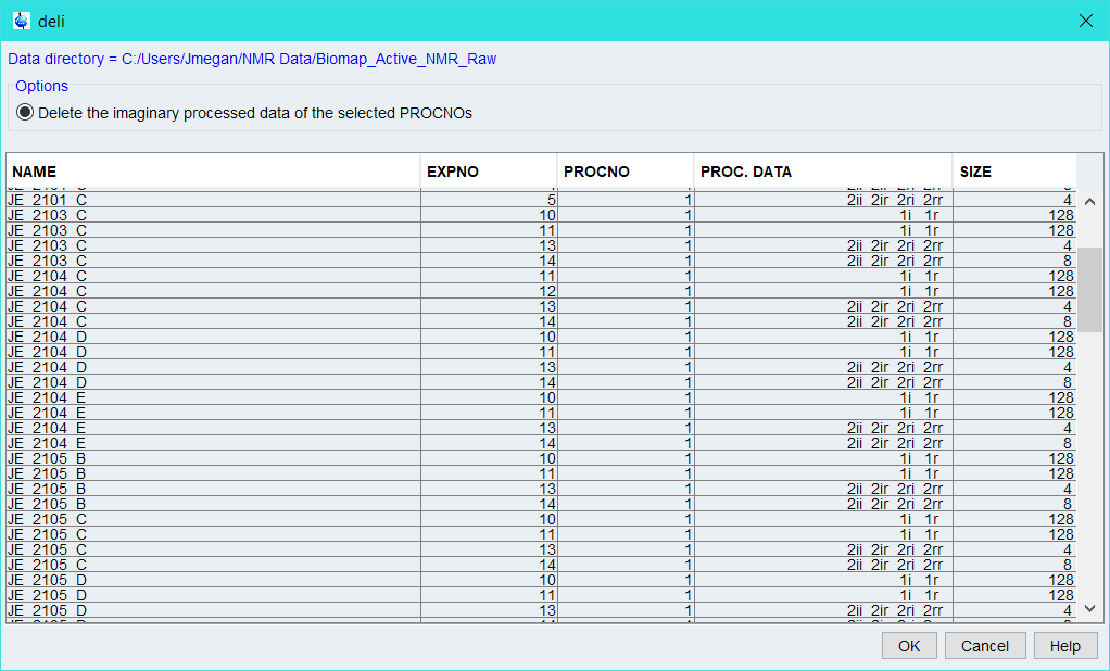
Before we jump in - there is a limit. I found this limit, repeatedly, when I was attempting to peak pick metabolomics 2D data. If you asked me if it could be done, I’d say yes - but I’d also say that it involves a lot more than what you may consider. For that reason, I have largely abandoned this single task in my automation pipelines and have opted for hand picking my data. However, if you’re working with pure molecules in a reasonable concentration, this is a much easier task. When I was originally looking into ways to make this a feasible task, a discussion between Clemens Anklin and John Hollerton put forth the idea of 80:20 confidence - that for around 80% of cases of automation, it’s possible to get great results, the other 20%, however, might prove challenging. For this reason, you should always manually check your data after an automated pipeline. In fact… you could even automate this…. but I digress.

Over the next few posts, I hope to shed some light on how to automate your NMR processing using Topspin. There exists some automation documentation in the Topspin Manual, but for the average user, the information can be overwhelming and it can take days of working through it to automate your first task. This is NOT a criticism! They are highly detailed and contain a lot of information that might be of interest. After these small blog posts, my hope is that you’ll be able to get started with automation in under 30 minutes and then progress to the manuals to fill in the gaps - once you know what you’re looking for, it’s easier to find.

Types of Automation

Topspin contains (at least) 3 different ways to automate your processing - and it’s accessible to all users, even on an academic license.

They are:

  • Macro Scripts

  • Python (Yes, REAL Python!)

  • Au Scripts/Macros

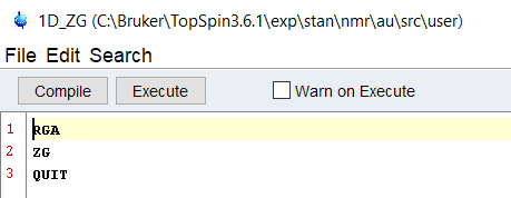
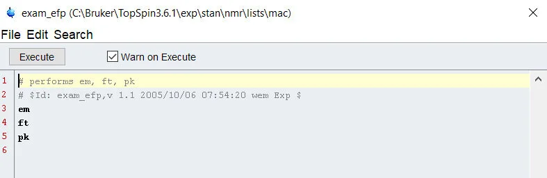
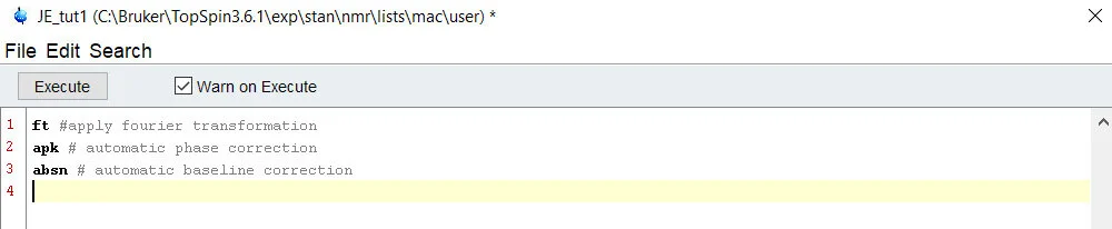
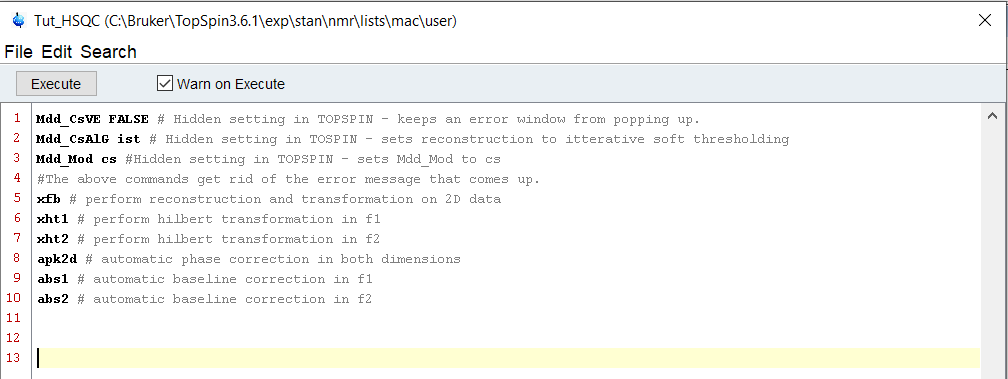
For the average user who knows nothing of coding, the simplest way to get started is by using Macros. I say this because when you program a macro in Topspin, you simply replace the human with a series of commands - if you already type things into the command line in topspin, you already know how to do it.

Other users, such as myself, who are familiar with Python will rejoice to learn that the python scripting in topspin can be used to read/write files - such as peak lists - or perform calculations on data and export the results. This can save you a massive amount of time in ensuring you have the right peak lists saved with the right file names in the right places, and if you already know basic python, Topspin’s python is really easy to use.

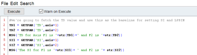
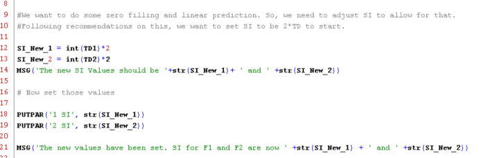
The last type, Au Scripts, are higher level programming scripts that must be compiled before execution. The code used recognizes topspin commands and C-language functions. The benefit, of course, is that it is extremely adaptable and very fast when compared head to head with python and it carries the same ability to export data easily. However, if you’ve not used a C based language, it can take some getting used to.

There are other factors that play into what to decide to automate with, but I find that people use the tools they’re already familiar with - we all have a toolbox filled with screwdrivers, but we all have a favorite (mine happens to be an old Craftsman given to me by my grandfather). MestreNova has it’s own scripting ability, but I will not be going into this toolchest - it’s someone else’s set.

I hope to create a post every Tuesday for the next 3 weeks to highlight each of these options, how to use them, and some simple scripts to get you started.

NMR Sample Prep - Tips and Tricks Vol. 1

Simply put, you’re not going to get good data from a bad sample.

This is especially true when you are:

  • Sample Restricted (low amounts)

  • Working with mixtures

  • Live in a temperate rainforest….

So, it took me about 4 months of my life to chase down the sources of problems in my process when I was devising MADByTE. The number 1 problem: Water. Since we were working with DMSO, this solvent takes up water in almost real time - or real time if you live in Vancouver… So I spent a long time trying to minimize this problem based off of some tips from my lab mates. I’ve highlighted these tips alongside my process for getting samples ready to for the NMR.

Sample Limited? Use a Shigemi Tube.

It should be noted, we have a 5mm probe in our instruments. This is my experience with our instruments.

Shigemi Tubes are fantastic specialty NMR tubes that allow for you to manipulate the amount of solvent present in your mixture. Think of it this way - you have 200ug of your compound, and it’s in 550uL of solvent… You may not get a very good signal because the reciever gain is being set by the solvent peak (or…in Vancouver… the water peak). How can you get around this when you don’t have any more sample? Shigemi Tubes.

Shigemi Tubes are ‘matched’ to solvents which means that they are essentially invisible chunks of glass that your magnet can shim to. This means you can concentrate your sample in considerably less solvent and get an increased return on signal with the same mass of the sample. Cool right? Here’s a quick figure to show what I mean. Shigemi tubes essentially give you a huge boost in your signal coming from your compound when compared to the standard 5mm tube because you’re using the shape of the tube (and matched glass) to shim and solvent instead of just solvent with your precious compound floating outside of the detection coil! We’ve been able to minimize the amount of solvent we use to around 280uL for a Shigemi tube, but you can go lower if you don’t mind manual shimming.

 
NMR_Tube_Comparison.png
 

We’ve also tested 3mm tubes in a 5mm probe, and have found different results than other groups that claim it works well. Personally, I find that the ease of working with Shigemi tubes far outweighs the hassle of using a 3mm tube, and we find that the signal response from a sample in a given concentration is better using a shigemi tube. If you have the ability to use a 3mm tube, try it out. You may have different results.

Keeping Water Out

This is the big one for DMSO work. There are a few straight up recommendations that I can make that will help.

Use ampoules instead of larger bottles of solvent

This one is fairly obvious, but could be a more expensive option. If you don’t have to keep your solvents in a super dry environment or if you don’t have to constantly re-open them, it’s a win! Ampoules can be more expensive than their bulk option, but as a recommendation, you might want to reach out to several companies for bulk pricing. I’ve worked with one company in particular which was able to give us ampoules for less than their volumetric equivalent in bulk from standard suppliers. I’m not advertising - so just email me for the company name. As a bonus, they were able to get all of our ampoules from the exact same batch which means that they are very well suited for qNMR applications.

Place your samples AND NMR tubes on a schlenk line/high vac

You wouldn’t believe how much water can stick to glass - which is why a lot of labs keep their NMR tubes in the oven. Firstly, you shouldn’t do this. The NMR tubes can slowly warp over time due to glass being an amorphous solid - placing them in a hot environment can exacerbate this effect to the point of it being a noticeable problem. So dry the other way… vacuum! Synthetic labs usually have a spare schlenck line around, so you can simply put your NMR tubes and samples under vacuum with one of those. We then back-fill with Argon since it is heavier than atmospheric air and arrives dry - so water vapor has less of a fighting chance to be a problem there.

Use Glass Pipettes - But differently than you may think…

This is a way to quantitatively transfer solvent. There are a few ways to do it, but for now, think about how you prep a standard NMR sample. You’re not using plastic pipette tips right? Plastic leaching aside, wouldn’t it be great if you could though?

For a lot of different applications, you will want the same amount of solvent in an NMR tube - some people use Hamilton syringes to achieve this, others use a setup like the one below. However, I find that this is a good start, but I wanted more accuracy and precision. On top of that, we had a problem where the syringe was contaminated with formic acid…. so we saw formic acid in every sample we prepped with this method for quite some time….

 
pluringe.png
 

Building on this idea, but taking it in another direction, I came up with the idea to use a standard pipette to transfer as if I had a glass tip for the pipette. I’ve seen pipettes that have glass tips - non disposable and expensive tips - but we didn’t have access to those… Not to make it more complicated than it should be, I simply stuck a pipette onto a pipette - tested it for accuracy and precision - and was quite surprised by the results. Using the graduation of the standard pipette, I was able to achieve quantitative transfer of my samples and was using disposable glass pipettes as the tips. A cheap fix to a problem.

Pipette_Post.tif.jpg

“Pull” Your Glass Pipettes To Minimize Water

If you’re not making your own TLC spotters, or if you don’t work in a microbiology lab, you may not be familiar with this step. Basically, you can take a glass pipette (super inexpensive) and with a few seconds under a blowtorch or Bunsen burner, heat it up and ‘pull’ the pipette. This causes the glass to be pulled very thin - great for creating longer pipettes (the long ones are actually more expensive!). The new pipette is longer, and has a ‘bulb’ at the end of it, so simply break it in the middle and use the top half.

Breaking_Pipette.png

When you put everything together, you’ll find that not only are your spectra more clear (less water in the spectra), but you’ll be able to shim in considerably faster times by saving a shim file to your custom filling and starting your shimming from that point. Since your sample geometry is roughly the same, you’ll stand a good chance at completing shimming even faster.

Safety Notes:

  • When pulling pipettes, don’t wear disposable gloves, as these can melt to your hands and cause a worse burn than the fire itself may.

  • When working with an open flame, move all solvents away from your working space, and wear a flame retardant lab coat - 100% cotton at a minimum or Nomex if you can.

  • Ensure you’re wearing eye protection when working with the glass pipettes, as they can break small shards which have the ability to travel.

  • And lastly, the ‘pipette on a pipette’ technique creates a very long pipette. Take some time to become comfortable wielding it, and ensure you are not working too closely to others. A steady hand (or lack thereof) can make a big difference in your day.

Acknowledgements: Thanks to Jake Haeckl for taking my sketches of an NMR spinner and creating such a beautiful figure. Thanks to Kenji Kurita for not only warning me about sample prep, but giving some great tips on how to handle it. Thanks to Claire Fergusson for taking some of the photos.

Using SMART NMR - With Topspin

NMR users rejoice!

In 2017, the Gerwick lab published a paper on the use of their system called SMARTnmr which uses some really nice pattern matching techniques to point you to a compound you have based on similarities of the HSQC spectra. Sounds like a cool idea right? Well, they’ve spent a lot of time and effort over the last year and some change to get this system up for others to use and have expanded the library of spectra to over 50,000 compounds! So, give it a try at smart.ucsd.edu - The documentation currently is set up for Mestrenova users and gives step by step instructions on how to get your data into the system.

But what if you’re not using Mestrenova? Well, if you’re using Topspin, I have a solution for you:

To make it as easy as possible for these users to be able to import their data, I've created a small script that utilizes Topspin's native python environment to do the heavy lifting.

Note: you can try changing the directories, but I found that sometimes the permissions don't line up too well. To circumvent this, the script puts peak lists a folder in the Bruker directory on your hard drive named SMART Peak Lists.You must change the directory to the relevant Mac directory if you are not on windows.

Step by Step on how to get these to work:

  1. Navigate to your Topspin directory (in windows, this is "C:Bruker")

  2. Create a new folder called "SMART Peak Lists"

  3. Open Topspin and type 'edpy' - hit enter

  4. In this dialog, go to the top right corner where it says "Source = [ combo bar filled with a few things] "

  5. Select the option in the combo box that ends with /py/user

  6. Go to File->New and name the script what you want (Hint: you can directly call the script from the input bar from now on, so call it something easy - I called mine SMART.py)

  7. Copy the code into the box and hit save.

  8. Open a data set that is peak picked to your satisfaction and type the name of your script into the input bar and hit enter. (I.E. 'SMART')

  9. If you do NOT get an error message, it should say 'SMART.py: finished' in the lower left corner.

  10. Navigate to the directory where your lists are stored.

  11. You'll see the sample name of your open data set followed by "_Peaks.csv"

  12.  Submit them into the website and rejoice.

After the first success, you'll be able to simply open a data set and type 'SMART' and your lists will be generated and given the right sample name, ready for the SMART server.

The Script:


import csv, os

curdat = CURDATA()

Peaklist = GETPEAKSARRAY()
SMART_PATH = os.path.abspath("C:\Bruker\SMART Peak Lists") #This is what you change if you are on MAC or wish to give the directory a different name.

Dest_Path=os.path.join(SMART_PATH,str(curdat[0])+'_Peaks.csv')

with open(Dest_Path, 'w') as csvfile:
    fieldnames = ['1H', '13C']
    writer = csv.DictWriter(csvfile,fieldnames=fieldnames,lineterminator = '\n')
    writer.writeheader()
    for peak in Peaklist:
        proton = round(peak.getPositions()[0],2)
        carbon = round(peak.getPositions()[1],1)
        writer.writerow({'1H':proton,'13C':carbon})

Hello World

MADByTE is a tool built for community development of NMR metabolomics, and that can be complicated.

There are a lot of factors that had to be considered for the development of MADByTE and other NMR metabolomics platforms - sample complexity, pulse sequence selection, peak picking, and automation of processing -just to name a few. Many of these small ‘huh…wish I knew that’ issues are worth discussion and I hope to provide a place to chat about them in the context of MADByTE’s development and usage.

There are already some wonderful tools and blogs out there, namely Stan’s NMR Blog and Glen Facey’s University of Ottawa NMR Blog, both of which have helped me figure out what the heck I’ve messed up and how I can improve it. There are other places to learn out there as well, such as The Resonance, which is a great example of Bruker’s outreach to learning and improving NMR as a research tool. When I can, I’ll post about a problem, how I solved it, and where I found the information from.

One truth I’ve learned though this process is just how much the community cares about developing new ideas, and how willing they tend to be in developing them into usable tools. People who - I thought I had no business talking to yet - have taken the time at conferences to discuss some of the challenges and be candid about the limitations they see. These problems are hard, and the willingness to share strategies have helped to catapult this project into fruition, and for that I’m eternally grateful.